Error in Multiplication Formula in MS EXCEL

Asked By 30 points N/A Posted on -
qa-featured

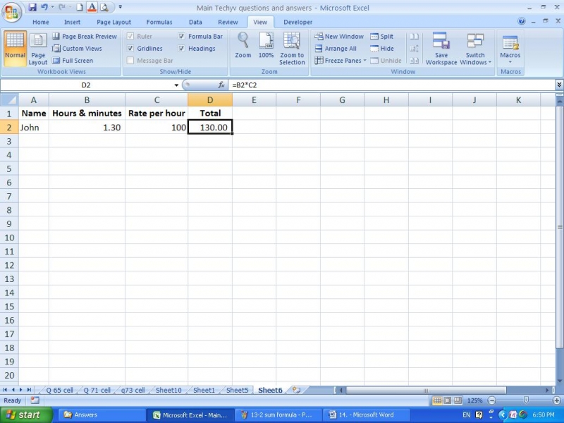
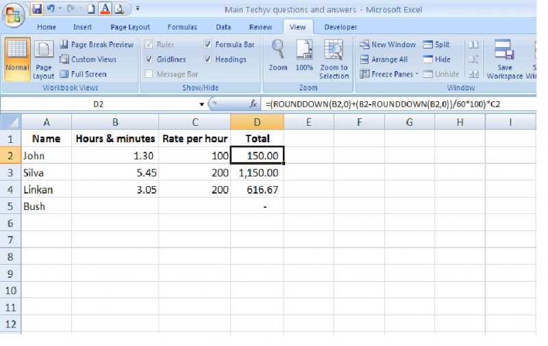
I have a worksheet that shows total hours and minutes worked, along with the hourly pay rate.

When I multiply these vales, I don't get the result I'm looking for.

What's wrong?

SHARE
Best Answer by Sherin Viluel
Answered By 80 points N/A #155105

Error in Multiplication Formula in MS EXCEL

qa-featured

In doing multiplication on Excel, you must use the symbol asterisk or * instead of “x”.

Also, the equal sign should be at the start of the formula instead of after.

Try the following to create a table with multiplication formula for your Excel spreadsheet:

  1. Click into the cell you would like to formula to be
  2. Click on the formula bar which is found at the top of Excel
  3. Type the following formula: = B15 * C15 wherein the B is the letter of the columns you’d like to multiply, and 15 is the number of row where the item you’d like to multiply is placed
  4. Hit enter

For further assistance or reference you may go here to or check this link.

Best Answer
Best Answer
Answered By 0 points N/A #155106

Error in Multiplication Formula in MS EXCEL

qa-featured

You can arrive at a solution in this way.

We will just take an example,

When the time is 1 hour and 30 minutes (assume that you have mentioned it as 1.30) and the hourly rate in 100 the total value should be 150.

However, in you excel you do not get that result (150) instead you get the result as 130 as follows.


The reason for the above result is, excel does not understand the .30 as 30 minutes or as half an hour. Instead it will understand it as 30 out of hundred. (30/100)

In order to get the result that you expect I will give you a formula that you can apply on the result column.

The formula is,

=(ROUNDDOWN(B2,0)+(B2-ROUNDDOWN(B2,0))/60*100)*C2

Important: you should apply this formula to Cell D2 if the hours and minute is cell B2 and the hourly rate is in cell C2.However, you can drag it down to any rows which you want.

Then you will be able to get the result you expected as shown in the following image.

Related Questions