Make Excel Import Data from Other Sheet

Asked By 0 points N/A Posted on -
qa-featured

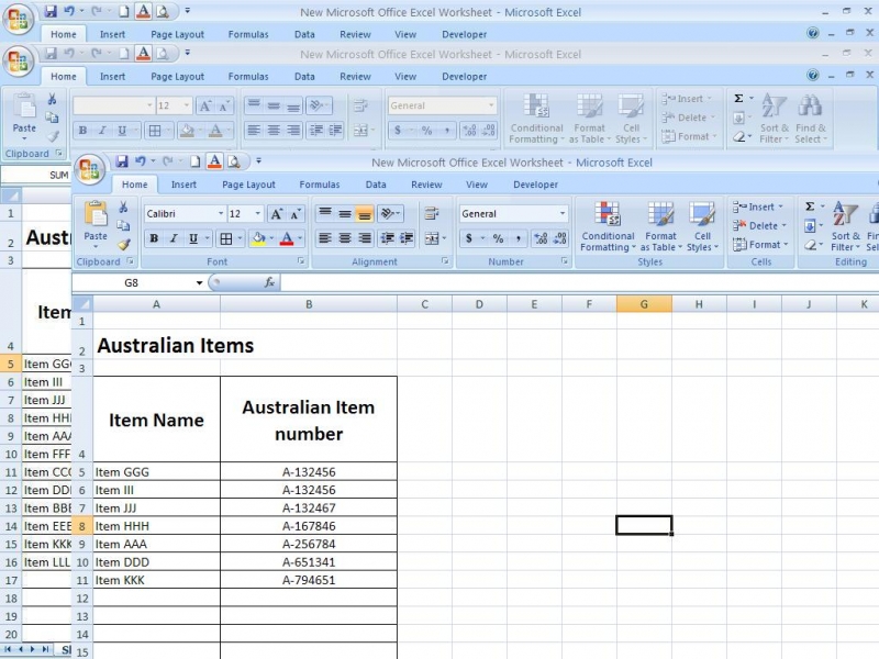
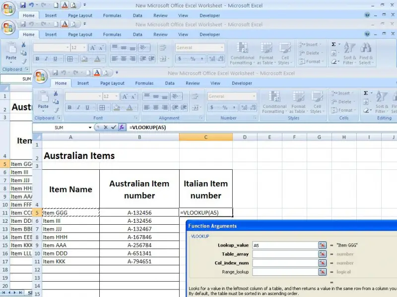
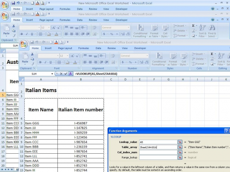
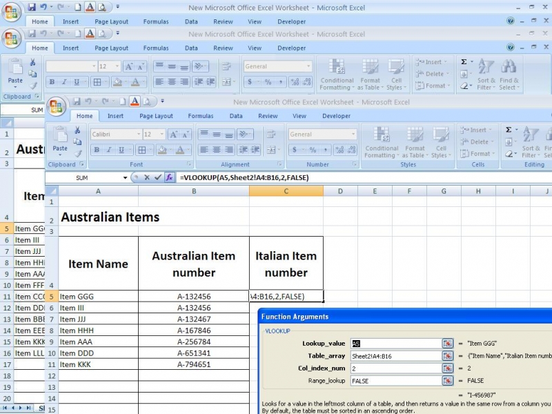
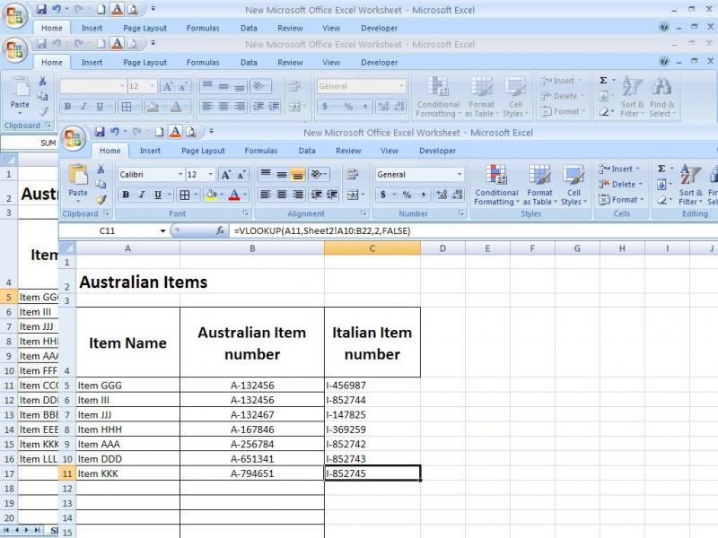
I have a worksheet with lots of item numbers and other forms of data from our Australian website. On my other worksheet, I have the item numbers from Italy and the correlating Australian items.  What I want to do is to create a formula that will automatically fill the correlating Italy item numbers into an empty column on the primary worksheet. I don’t have any clues on how to do this, but doing it manually will definitely take me ages to finish. So, is there another way to have the Excel import data from another sheet to pull the correct item number across and make a complete data sheet? I’d be really grateful to those who can answer.

SHARE
Best Answer by Sherin Viluel
Answered By 20 points N/A #114296

Make Excel Import Data from Other Sheet

qa-featured

Microsoft Query can be used to import excel data from one excel sheet to another. Please follow the procedure below if you are using Microsoft Office 2007:

·         Go to Data Menu on Excel

·         Click From Other Resources then choose From Microsoft Query 

·         Choose Excel Files on the Choose Data Source window then click OK.

·         Select the file on which you will be copying the data from. Sheets of the file will be listed and you would be able to select which table you wish to import. Data will be filtered and sorted.

·         Save the query and select button that says ‘Return Data to Microsoft Excel’.

·         Click on Finish and the import of data will start.

Best Answer
Best Answer
Answered By 0 points N/A #114297

Make Excel Import Data from Other Sheet

qa-featured


You are able to do this very quickly and easily by using the Microsoft excel function called “ VLookup”.

I will take as an example in the first sheet which includes data of Australian items contains the following columns.


In the second sheet I will enter data of the Italian Items.


Now on the sheet1 in column C, I will put a heading as “Italian Item Number”. Then use the Vlookup function as follows.

Go to the column C5 and type the “=vlookup(”.

Click on the “fx” button then the vlookup window will be appeared.


Click on the red arrow in the lookup value box and select the A5 cell.

Again click on the red arrow then the Vlookup window will be opened.


Now click on the red arrow in table array and go to the sheet 2 (Italian Items) and select the entire table from Item name column.


Now type number “2” in Column index_num and type FALSE in Range Lookup and click ok.


Now copy the formula in Cell C5 in to below cells. Then Italian item numbers have been displayed in that column as follows.


Related Questions