Asked By
susan1962
0 points
N/A
Posted on - 09/23/2011

Recently I set up a Pivot Table in Excel which shows inventory purchased and inventory sold for my business. I would like to add a simple calculation in the Pivot Table showing the difference between the amount purchased and amount sold, giving me my on hand inventory.
Can a calculation be added to a Pivot Table once it has been set up?
|
Item |
Data |
Total |
|
|
Blue Candle |
Sum of Purchased |
50 |
|
|
|
Sum of Sold |
12 |
|
|
Blue Votive |
Sum of Purchased |
75 |
|
|
|
Sum of Sold |
42 |
|
|
Cream Votive |
Sum of Purchased |
75 |
|
|
|
Sum of Sold |
27 |
|
|
Gold Candle |
Sum of Purchased |
50 |
|
|
|
Sum of Sold |
2 |
|
|
Green Candle |
Sum of Purchased |
50 |
|
|
|
Sum of Sold |
11 |
|
|
Red Candle |
Sum of Purchased |
50 |
|
|
|
Sum of Sold |
27 |
|
|
White Votive |
Sum of Purchased |
75 |
|
|
|
Sum of Sold |
38 |
|
|
Total Sum of Purchased |
425 |
|
|
Total Sum of Sold |
|
159 |
|
Calculating Data in an Excel pivot table
Even though the Pivot Table has already been set-up, through drag-n-drop, criteria can be manipulated. The process are as follows:
-
To change the “field formula” you have to click on the PIVOT TABLE on the PIVOT TABLE “toolbar”, and in the FORMULAS menu, hit CALCULATED FIELD.
-
Select the category or group of data that needs changing, a FORMULA box will appear after clicking the name of the group or field.
-
Change the formula as you desire and hit MODIFY. And then hit OK.
If you want to change the formula of an item you have to:
-
Click or choose the group or field where the item that you want to change is.
-
Then hit PIVOT TABLE on the PIVOT TABLE toolbar and instead of CALCULATED FIELD choose CALCULATED ITEM in the formula menu.
-
Highlight the name of the item that needs to be changed, change the formula in the FORMULA BOX.
-
Click MODIFY, then OK.
Hope this helps.
Calculating Data in an Excel pivot table
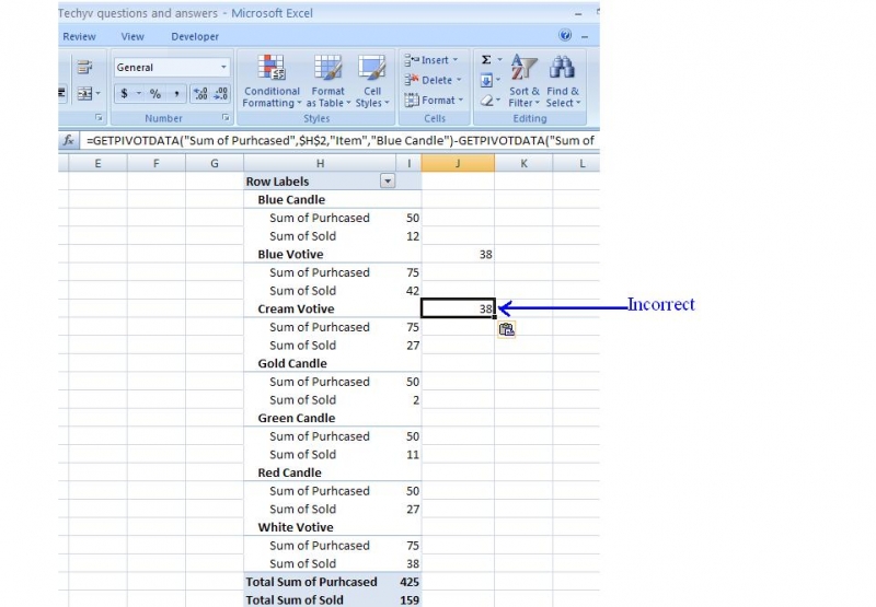
In excel it is impossible to add calculation or formula directly to a pivot table. You can add a calculation in to a cell which is out of the pivot table as shown in the below image but you will not be able to copy that formula to the other cell.
If you copied it to other cells, it will show the same result which is in the first cell.
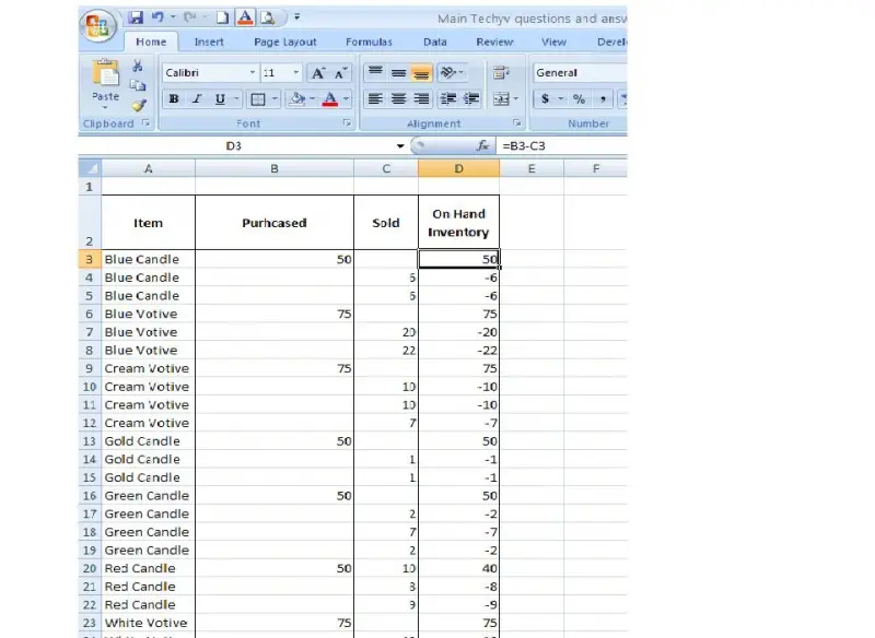
However, you can add a calculation to the data source which you can get the on hand inventory and then it is possible to add that field to pivot table as follows.
First get the on hand inventory to the data source by adding a new column as on hand inventory and type a formula to get the balance inventory (purchase quantity – sold quantity).
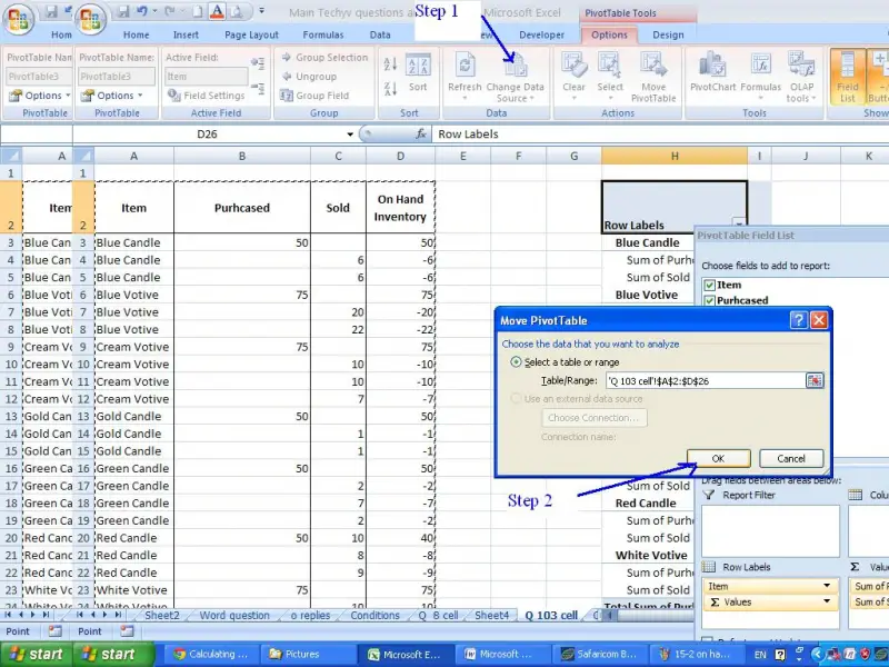
Then go to the “options” tab and click on the “change data source” on Data section (Step 1).
Then select the entire data source including new on hand inventory column and click ok (step 2).
Then go to the “options” tab and click on the “Field list” in show/hide section.

Drag the “on hand inventory” field and put it to Values field.
Make the “on hand inventory “field to sum format.
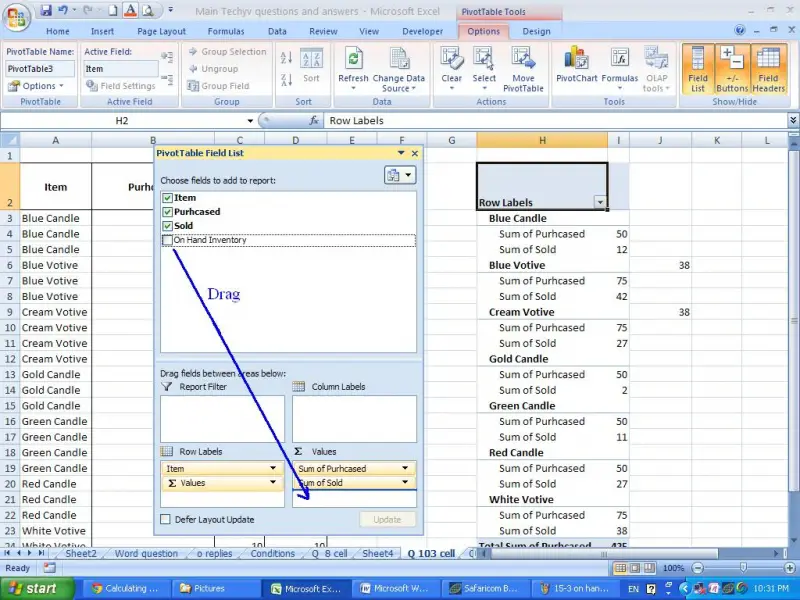
Now you will be able to see the “on hand inventory” column in pivot table as follows.


